This practical lecture is again based on Jupyter Notebooks. You can see and download the notebook corresponding to today here. For completeness, please also download the following set of Python files, which will illustrate the use of Jupyter notebooks in combination with Spyder: [1], [2], [3]. Please store them in the same folder as where you put the notebook.

Note that we discuss Linear Regression in Theoretical Lecture 6. For this reason, we will only be using them alsmot as a black-box today, to familiarize ourselves with sk-learn for regression tasks.

Here is the plan for today:

1. Motivation and Goals. Machine Learning for Supervised Classification and Regression

   1. Difference between Classification and Regression
   2. Difference between Generative and Discriminative models
   3. Aside: Working from Spyder
   4. Quick overview of scikit-learn

2. Bayesian Classification: a Bit of Theory

3. Naive Bayes Classifier Implementation

   1. From scratch
   2. Using scikit-learn

4. Linear Regression: a (tiny) Bit of Theory

5. Linear Regression Using scikit-learn

6. Homework 😱

7. Sources and References

1.- Motivation and Goals. Machine Learning for Supervised Classification and Regression

As you will know, this course is all about about making predictions out of data and annotations. But there are several different kinds of predictions, and hence several tasks that we can solve. Among the most fundamental ones are Supervised Classification and Supervised Regression.

Note: The term supervised refers to the fact that we assume we have data with annotations. A different kind of models exist related to the situation where there is no annotations, and the goal is to extract some useful information out of the available (unlabeled) data. This is called unsupervised learning.

For instance, we could think of a dataset with customer preferences regarding certain products. Could we group a given pool of users into several subgroups that behave similar among them, but differently with respect to the other subgroups? This task is known as clustering, and we will be working on it in future lectures. But for now, we assume for each example in our dataset, we know the corresponding quantity of interest.

1.1 - Difference between Classification and Regression

Classification: in your data every examples is associated to two or more classes. You want to learn from this labeled data how to predict the class of new unlabeled data.

Example: Given a set of lung CT scans, a doctor has annotated each of them after examination, specifying whether they show or not signs of lung cancer.

Regression: In this case, the output of your model is is not a discrete label, but a real number.

Example: given a training set in which you have examples of red and white globule concentration, predict the amount of blood pressure. In this case, the output (blood pressure) is not a single label, but a number.

Both classification and regressoin are supervised learning problems, since there is labeled data available. However, the discrete nature of classification, as opposed to continuous for regression, require different types of learning models.

1.2 - Difference between Generative and Discriminative models

In (supervised) learning we always have a dataset of examples with associated labels. However, we do not usually feed our models with the raw data (with a super-relevant exception that we will see later in this course).

For instance, imagine I have a dataset of all the movies I watched in 2016 and 2017, and each movie is tagged with a label indicating whether I liked it or not. If I want to build a model that takes a new movie and predicts if I will like it or not, I am not going to give to my classifier every frame of the movie and let it process it. Rather I am going to extract some key information summarizing the movie, such as genre, actors and actresses, duration, soundtrack, etc. We call these key informative traits of our data features, and their selection is

Imagine now that I decided that with the duration and rating of the movie in IMDB, I can already describe the movie in such a way that I can build a classifier for my problem. We can build the following plot:

import numpy as np
import matplotlib.pyplot as plt
from sklearn.datasets import make_blobs
%matplotlib inline

# create some synthetic data
n_samples = 100
n_features = 2
movies_mean = [[1.5, 7], [2, 8]] # [mean_movie_duration, mean_IMDB_score]
movies_std = (0.25, 0.25) # [std_movie_duration, std_IMDB_score]
movies, like_it_or_not = make_blobs(n_samples, n_features, movies_mean, movies_std)


movies_I_liked = movies[like_it_or_not==1]
movies_I_disliked = movies[like_it_or_not==0]

# plot data points
plt.scatter(movies_I_liked[:,0],movies_I_liked[:,1], marker = 'o', color = 'g', label = 'Liked');
plt.scatter(movies_I_disliked[:,0],movies_I_disliked[:,1], marker = 'o', color = 'r', label = 'Disliked');
plt.xlabel('duration');
plt.ylabel('IMDB rating');
plt.legend();
plt.show()

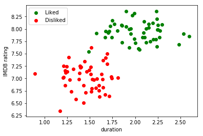
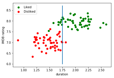
Roughly speaking, what a discriminative model will do in this case is trying to find something called decision boundary that allows us to tell apart movies I liked from movies I did not like.

For instance, it could be a simple linear decision boundary, a predictive model stating that if the movie has a duration of less than 1,75 hours, I will like it:

x = 1.75*np.ones(100)
y = np.linspace(6.0,8.7,100)
plt.scatter(movies_I_liked[:,0],movies_I_liked[:,1], marker = 'o', color = 'g', label = 'Liked');
plt.scatter(movies_I_disliked[:,0],movies_I_disliked[:,1], marker = 'o', color = 'r', label = 'Disliked');
plt.xlabel('duration');
plt.ylabel('IMDB rating');
plt.legend();
plt.plot(x,y, lw = 2)
plt.show()

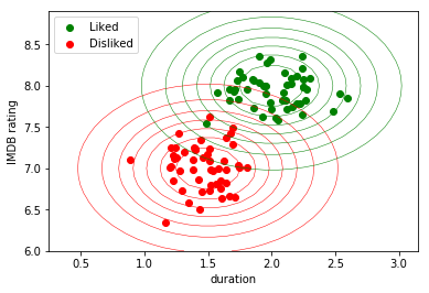
In contrast, a generative model would try to find a model that explains the way the data was generated for both classes (liked/disliked). After these models have been built, given a new example, we can inspect which of the two models was more likely to have generated that example.

For instance, we could model both distributions (liked/disliked) as being generated by a Gaussian distribution. Since I created the above synthetic data, I already know that it comes from two different distributions, parametrized by $(\mu_1, \sigma_1) = (1.5, 7)$ and $(\mu_2, \sigma_2) = (2, 8),$ and I can for instance draw a nice contour plot:

from scipy.stats import multivariate_normal

rv = multivariate_normal([1.5, 7], [[0.25, 0], [0, 0.25]]) # normal distribution around (1.5, 7)
rv_2 = multivariate_normal([2, 8], [[0.25, 0], [0, 0.25]]) # normal distribution around (2, 8)

x_grid, y_grid = np.mgrid[0.25 : 3.25: 0.1, 6 : 9: 0.1]
pos = np.empty(x_grid.shape + (2,))
pos[:, :, 0] = x_grid; pos[:, :, 1] = y_grid

plt.contour(x_grid, y_grid, rv.pdf(pos), linewidths=0.5, colors = 'r')
plt.contour(x_grid, y_grid,rv_2.pdf(pos), linewidths=0.5, colors = 'g')

plt.scatter(movies_I_liked[:,0],movies_I_liked[:,1], marker = 'o', color = 'g', label = 'Liked');
plt.scatter(movies_I_disliked[:,0],movies_I_disliked[:,1], marker = 'o', color = 'r', label = 'Disliked');
plt.xlabel('duration');
plt.ylabel('IMDB rating');
plt.legend(loc = 'upper left');
plt.show()

The fact that we know the model that the data distribution follows has several advantages. We can for instance sample, i.e. generate, new data points for each of the two classes. This is the origin of the term generative.

Quoting David Duvenaud:

Generative modeling loosely refers to building a model of data, for instance p(image), that we can sample from. This is in contrast to discriminative modeling, such as regression or classification, which tries to estimate conditional distributions such as p(class | image).

Generative models have several advantages and disadvantages with respect to discriminative ones. In a quick and dirty summary, they allow us to better understand if/how we are capturing the real-world distribution through our dataset, but they are harder to understand, implement, and scale-up to large quantities of data.

However, it is important to be aware of their existence. Today we will be discussing probably the simplest instance of a generative model for classification, namely Naive Bayes.

1.3 - Aside: Working from Spyder

At some point you may feel uncomfortable with the room that notebooks leave for playing with your code or organizing it. For instance, you will have noticed that there is lots of redundant code above.

At this link, I am attaching a series of files meant to reproduce the above example in Spyder. Please download them to your working folder, open them, and observe how the different import statements interact among them. You do not need to understand all this code does, but it is important that you understand the way it flows.

By the way, you can also write code in a separate .py file, import it, and use it from your notebook, as long as they both are in the same folder. See the example below:

import daco_visualizations as dv
dv.plot_vertical_line(1,2,4)

1.4 - Quick overview of scikit-learn

The main Python library for machine learning is called scikit-learn, often abbreviated sklearn. We have already used a function belonging to sklearn above, namely make_blobs().

Sklearn exposes to the user useful objects and functionalities to solve machine learning problems, such as:

• Classification
• Regression
• Clustering
• Dimensionality Reduction
• Model Selection
• Preprocessing

Sklearn even brings a module with some datasets with it that can be used to illustrate machine learning problems. There are specific functions to load those datasets available. Let us load the famous Iris flower dataset, consisting of $50$ observations of three species of Iris, namely Iris setosa, Iris virginica and Iris versicolor. In this case, four features are measured from each sample: length and the width of the sepals and petals. The label in this case is the kind of iris flower, and it consists of a 3-class classification problem.

Let us load the dataset, keeping only the first two classes for demonstration purposes:

from sklearn import datasets
import numpy as np
iris = datasets.load_iris()

subset = np.logical_or(iris.target == 0, iris.target == 1)

X = iris.data[subset]
y = iris.target[subset]

The (X,y) subdataset has now two classes and 50 elements on each one. Each example is described by 50 features.

print(X[y==0].shape)
print(X[y==2].shape)
print(X[0,:], y[0])
print(X[60,:], y[60])

How does sklearn exposes its tools? Through interfaces with the user. The main ones are:

Model:

score = obj.score(data)    

Estimator:

estimator = obj.fit(data, targets) 

Predictor:

prediction = obj.predict(data) 

Transformer:

new_data = obj.transform(data) 

For instance, given the above dataset, you can instantiate a model. The following is an example of a linear classifier, that we will discuss in class next week, but for the moment focus only on the “computational” side of this:

from sklearn.linear_model import LogisticRegression

model = LogisticRegression()

print(type(model))

You can now use the Estimator interface to learn the parameters that best fit a model to your data and labels:

model.fit(X, y)

With a fitted model, you can for instance check if it is performing adequately (in this case the solution was perfect):

model.score(X, y)

Once the model has been fitted, you can also use it to predict labels on new data. You can even do this for a batch of new examples in one single line:

model.predict([[5,4,2,1], [5,2,4,1]])

We will be covering most of the other functionalities that sklearn gives you in the remaining lectures. For those who are curious, the documentation (which is really nice and full of examples) can be found here.

2.- Bayesian Classification: a Bit of Theory

You have already seen in the theoretical lectures Bayes’ formula:

$$\mathcal{P}(A \ | \ B) = \frac{\mathcal{P}(B \ | \ A) \cdot \mathcal{P}(A)}{\mathcal{P}(B)} \ \ \ \ \ (1)$$

Which you should interpret as the posterior probability of $A$ given $B$ being proportional to the posterior probability of $B$ given $A$ multiplied by the probability of the prior $A$. Or in plain English, that your knowledge on a given event $\mathcal{P}(A)$ is updated after performing an experiment $B$ with a multiplier $\mathcal{P}(B \ | \ A)$, becoming $\mathcal{P}(A \ | \ B)$.

But, how do we use Bayes’ rule in practice to design a Bayesian classifier?

Consider a classification problem with $K$ possible classes, in which the data has been represented by $\mathbf{x} = (x_1,x_2, \ldots, x_N)$, and we denote the classes as $\omega_k$, $1\leq k\leq K$. In the absence of training data, the simplest decision rule for classifying a new sample would be to pick the class $\hat{\omega}$ for which the prior probability (which you have from the beginning and states your opinion of the world before you see the training data):

$$\hat{\omega} (\mathbf{x}) = \underset{k}{\operatorname{argmax}} \left[\mathcal{P}(\omega_k) \right]_{k=1}^K$$

For instance, if you know that a particular type of cancer has an incidence of $0,1\%$ in the population, when a new patient arrives, you could tell her that she has cancer with probability $p=0.001$. This is a quite poor diagnosing strategy.

However, our training data gives us a way to model $\mathcal{P}(\mathbf{x} \ | \ \omega_k)$, since we know the labels associated to each example. We will see below the way we build that model from the available data.

But for now, consider in this context Bayes’ rule: it gives us a way of updating our knowledge. Formula (1) is re-written now as:

$$\mathcal{P}(\omega_k | \mathbf{x}) = \frac{\mathcal{P}(\mathbf{x} | \omega_k) \times \mathcal{P}(\omega_k)}{\mathcal{P(\mathbf{x})}} \ \ \ \ \ (2)$$

It is the left-hand side of this formula, i.e. the Posterior probability, that we need in order to classify new data into one of our classes. What do we have to build this?

• The Likelihood $\mathcal{P}(\mathbf{x} | \omega_k)$, that we will extract from the training data.
• Our Prior $\mathcal{P}(\mathbf{\omega_k})$ of how is data actually distributed into our classes in our experience.
• The Evidence $\mathcal{P(\mathbf{x})}$, a term that you can consider just a simple scaling factor to ensure that the posterior probability adds up to $1$ and thus it is a correct probability distribution.

In this context, there is a simple decision rule, called MAP (Maximum A Posteriori probability), that allows us to classify new data: assign to $\mathbf{x}$ the class $\hat{\omega}_{MAP}$ that receives the greatest amount of posterior probability $\mathcal{P}(\omega_k | \mathbf{x})$ according to $(2)$. Mathematically, this is formulated as:

$$\hat{\omega}_{MAP} (\mathbf{x}) = \underset{k}{\operatorname{argmax}} \left[\mathcal{P}(\omega_k|\mathbf{x})\right]_{k=1}^K = \underset{k}{\operatorname{argmax}} \left[\mathcal{P}(\mathbf{x}|\omega_k) \cdot \mathcal{P}(\omega_k)\right]_{k=1}^K,$$

where we have already dropped the evidence in the denominator, since we are interested in finding the a-posteriori maximizing class, and $\mathcal{P}(\mathbf{x})$ will be a factor affecting equally all classes (it does not depend on $k$).

Since it is easier to maximize a sum than to maximize a product, we prefer to split the above MAP solution into:

$$\hat{\omega}_{MAP} (\mathbf{x}) = \underset{k}{\operatorname{argmax}} \left[\log(\mathcal{P}(\mathbf{x}|\omega_k)) + \log(\mathcal{P}(\omega_k))\right]_{k=1}^K \ \ \ \ \ (3)$$

And now it comes the magic: we are going to assume that the distribution of each class $k$ can be modeled through a Gaussian distribution parametrized by a mean and a standard deviation given by $(\mu_k, \Sigma_k)$:

$$ \begin{align} \mathcal{P}(\mathbf{x} | \omega_k) &\sim \mathcal{N}(\mathbf{x} \ | \ \mu_k, \Sigma_k) = \frac{\displaystyle 1}{\displaystyle (2\pi)^{N/2}} \cdot \frac{\displaystyle 1}{\displaystyle |\Sigma_k|^{N/2}} \cdot \mathrm{exp}\left(\displaystyle \frac{-1}{2} \cdot (\mathbf{x} - \mu_k)^T \cdot \Sigma_k^{-1} \cdot (\mathbf{x}-\mu_k)\right), \ \ \ 1\leq k \leq K, \end{align} \ \ \ \ \ (4) $$

where $|\cdot|$ represents the determinant of a matrix. Please note that $N$ is the dimension of our problem, in terms of the number of features that describe the data, i.e. $\mathbf{x} = (x_1,\ldots,x_N)$.

Aside: Normal Distribution

If you are familiar with the general formulation of a Gaussian (normal) distribution in many dimensions, you can skip the following paragraphs.

The above multi-dimensional distribution has an easy interpretation, as usual in maths, once you look at particular cases in low dimensions. This allows you to map the new ideas to your previous knowledge (Bayes rule attacks again?). Recall that a Normal distribution in 1D is defined as:

$$ \mathcal{N}(x \ | \ \mu, \sigma) = \frac{\displaystyle 1}{\displaystyle \sqrt{2\pi\sigma}} \cdot \mathrm{exp} \left(\displaystyle -\frac{(x-\mu)^2}{2\sigma^2}\right) $$

Which can be rewritten as: $$ \mathcal{N}(x \ | \ \mu, \sigma) = \frac{1}{(2\pi)^{1 / 2}} \frac{1}{\sigma^{1 / 2}} \cdot \mathrm{exp} \left(\displaystyle \frac{-1}{2} \cdot (x-\mu) \cdot \frac{1}{\sigma^2}\cdot (x-\mu)\right) \ \ \ \ \ (5) $$ And here, $x, \mu, \sigma$ are simply real numbers.

But what if you want to model random variables that depend on two numbers, i.e., how can we define a bivariate normal distribution? In this case, we would have $\mathbf{x} = (x_1, x_2)$, $\mu = (\mu_1, \mu_2)$ and the standard deviations $(\sigma_1, \sigma_2)$ are represented into the covariance matrix, that captures the correlation between both variables:

$$\Sigma=\begin{pmatrix} \sigma_{1}^2 & \sigma_1\sigma_2 \\ \sigma_1\sigma_2 & \sigma_{2}^2 \end{pmatrix},$$

with $|\Sigma|$ representing its determinant, which is another real number.

If you stare a while to formula (5), comparing it with (4), you should now see how and why one generalizes the other. If you still cannot see it clearly, I encourage you to replace $\mathbf{x}, \mu, \Sigma$ by actual values and do some paper and pen algebra.

---

Let us move forward in our goal to build a model that can classify new data. Remember the simple logarithmic rules:

$$\log(a\cdot b) = \log(a) + \log(b), \ \ \log(a^b) = b\cdot\log(a), \ \ \log(\exp(a))=a.$$

Inserting (4) into (3), we obtain:

$$ \hat{\omega}_{MAP} (\mathbf{x}) = \underset{k}{\operatorname{argmax}}\left(\frac{-1}{2} (\mathbf{x}-\mu_k)\Sigma_k^{-1}(\mathbf{x}-\mu_k) - \frac{N}{2}\log(2\pi) - \frac{1}{2} \log(|\Sigma_k|) + \log(\mathcal{P}(\omega_k))\right) \ \ \ \ \ (6)$$

The MAP decision rule tells us to select the class $k$ maximizing the above equation. This means that we can safely ignore the term in (6) that does not depend on $k$, since it is simply an added constant that won’t affect who is the “maximizating” class:

$$ \hat{\omega}_{MAP} (\mathbf{x}) = \underset{k}{\operatorname{argmax}}\left(\frac{-1}{2} (\mathbf{x}-\mu_k)\Sigma_k^{-1}(\mathbf{x}-\mu_k) - \frac{1}{2} \log(|\Sigma_k|) + \log(\mathcal{P}(\omega_k))\right) \ \ \ \ \ (7)$$

This formula already gives us a classifier. We would estimate $\mu_k$ and $\Sigma$ by computing the different mean and standard deviations of each class on our training data, and then insert them into (7).

There are however further simplifying assumptions that we can make. We can assume that all the different classes are spread in the same away around their mean values, i.e. $\Sigma_k = \Sigma \ \forall k$. Then, the MAP Bayesian classifier is simplifed as:

$$ \hat{\omega}_{MAP} (\mathbf{x}) = \underset{k}{\operatorname{argmax}}\left(\frac{-1}{2} (\mathbf{x}-\mu_k)\Sigma^{-1}(\mathbf{x}-\mu_k) + \log(\mathcal{P}(\omega_k))\right)$$

Yet a more restrictive assumption is to suppose that there is independence between the different features describing the data $\mathbf{x}$. In this case the covariance matrix is diagonal, $\Sigma_k = \sigma^2 \mathrm{Id}$, hence $|\Sigma_k| = \sigma^2$, and the classifier is even more simple:

$$ \hat{\omega}_{MAP} (\mathbf{x}) = \underset{k}{\operatorname{argmax}}\left(\frac{-1}{2\sigma^2} (\mathbf{x}-\mu_k)(\mathbf{x}-\mu_k) + \log(\mathcal{P}(\omega_k))\right) \ \ \ \ \ (8)$$

The term appearing in the right part of equation (X) is a particularly relevant mathematical entity called Mahalanobis distance. Let us analyze it.

Consider two $N$-dimensional points $\mathbf{x} = (x_1, \ldots, x_N)^T$ $\mathbf{y} = (y_1, \ldots, y_N)^T$. The standard Euclidean distance between them is given by:

$$ \mathrm{dist}(\mathbf{x}, \mathbf{y}) = | \mathbf{x} - \mathbf{y} |_2 = \sqrt{ (x_1 - y_1)^2 + \ldots + (x_N - y_N)^2} $$

Notice that this expression can be related to the usual vector product operation as follows:

$$ \mathrm{dist}(\mathbf{x}, \mathbf{y})^2 = \left(\mathbf{x}-\mathbf{y}\right)^T \cdot \left(\mathbf{x}-\mathbf{y}\right) $$

The Mahalanobis distance between those to vectors is a generalization of the squared Euclidean distance:

$$ \mathrm{dist}_{Mahalanobis}(\mathbf{x}, \mathbf{y}) = \left(\mathbf{x}-\mathbf{y}\right)^T \cdot A \cdot\left(\mathbf{x}-\mathbf{y}\right), $$

where we have introduced an $N\times N$ matrix in between both products. Note that if $A$ is the identity, both distances measure the same. However, if $A$ is a different matrix, interesting things can happen!

Example:

Let us define two bivariate normal distributions with means $\mu_1=(0,0)^T$ and $\mu_2=(1,1)^T$. Consider also that the covariance matrixes for each distribution are given by:

$$\Sigma_1 = \Sigma_2 = \begin{pmatrix} \sigma_1^2 & 0 \\ 0 & \sigma_2^2 \end{pmatrix}= \begin{pmatrix} 0.5 & 0 \\ 0 & 2 \end{pmatrix}.$$

We can plot their contours with a code similar to the one we used in the introduction:

mu_1 = np.array([0,0])
mu_2 = np.array([1,1])

sigma_1 = 0.5
sigma_2 = 2

sigma = np.array([[sigma_1,0],[0,sigma_2]])

rv = multivariate_normal(mu_1, sigma) # normal distribution around (mu_1)
rv_2 = multivariate_normal(mu_2, sigma) # normal distribution around (mu_2)

x_grid, y_grid = np.mgrid[-3 : 3: 0.1, -3 : 4: 0.1]
pos = np.empty(x_grid.shape + (2,))
pos[:, :, 0] = x_grid; pos[:, :, 1] = y_grid

plt.contour(x_grid, y_grid, rv.pdf(pos), linewidths=0.5, colors = 'red');
plt.contour(x_grid, y_grid,rv_2.pdf(pos), linewidths=0.5, colors = 'green');
plt.plot(mu_1[0], mu_1[1], marker='o', markersize=10, color='red');
plt.plot(mu_2[0], mu_2[1], marker='o', markersize=10, color='green');
plt.plot(1, 0, marker='o', markersize=10, color='blue');
plt.axes().set_aspect('equal', 'datalim') # This line here guarantees 1:1 aspect-ratio

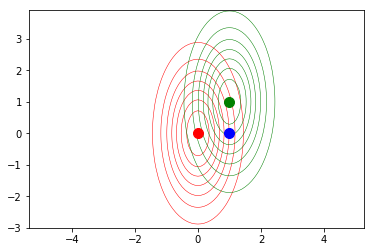
Let us compute the Euclidean distance between each of the two distribution centers and the point $(0,1)^T$, plotted in blue in the previous snippet.

def squared_dist(x,y):
    return np.sqrt((x-y).dot(x-y))

new_point = np.array([0,1])
print(squared_dist(mu_1,new_point))
print(squared_dist(mu_2,new_point))

Now, implement and compute the Mahalanobis distance.

def mahalanobis_dist(x,y,A):
    return (x-y).dot(A).dot(x-y)

print(mahalanobis_dist(mu_1, new_point, sigma))
print(mahalanobis_dist(mu_2, new_point, sigma))

The idea is that according to the Euclidean distance, both mean distributions are equally far away from the blue point, while the Mahalanobis formulation weighs that distance by considering the “shape” of the distributions, enconded in the covariance matrix: the second (green) distribution is closer to the point. This implies that the second distribution is more likely to have generated the blue sample.

This simple idea is actually what a Naive Bayes classifier implements in the case of the last simplification above:

• Given training data, we model each class distribution via a normal distribution.
• Given a new point, we compare its distance with regard to each distributions with the Mahalanobis distance
• The closest distribution is the one most likely to have generated the new point, and we assign that class to it.

Note however that the Bayesian formulation also allows us to introduce our prior experience in the model via the term $\log(\mathcal{P}(\omega_k))$ from eq. (8).

3.- Naive Bayes Classifier Implementation

Let us see how can we implement the above ideas for classification tasks.

3.1 - From scratch

To experiment with real data, we are going to use the Pima Indian dataset, provided by the UCI Machine Learning repository, and described here. The dataset contains $768$ observations (from indian patients) of $8$ different features, and the task is to try to predict if the patient will suffer from diabets. This means we face a binary classification problem. The observed features are all real or integer variables:

1. Number of times pregnant
2. Plasma glucose concentration a 2 hours in an oral glucose tolerance test
3. Diastolic blood pressure (mm Hg)
4. Triceps skin fold thickness (mm)
5. 2-Hour serum insulin (mu U/ml)
6. Body mass index (weight in kg/(height in m)^2)
7. Diabetes pedigree function
8. Age (years)
9. Class variable (0 or 1)

We are going to use pandas for importing the data directly from the internet. pandas is another Python library, useful for data analysis, but you do not need to worry about it right now, we will immediately store the data into a numpy array.

import pandas as pd

df = pd.read_csv('https://archive.ics.uci.edu/ml/machine-learning-databases/pima-indians-diabetes/pima-indians-diabetes.data',
                 header=None)
df.columns = ['#pregnant', 'glucose', 'blood_pressure', 'thickness', 'insulin', 'body_mass_idx', 
              'pedigree', 'age', 'label']
df.head()

Notice that pandas contains useful functions to explore your data:

import pandas as pd

df.describe()

Let us store the features and the labels in separate numpy arrays:

dataset = np.array(df)
print(df.shape)

features = dataset[:, :8]
labels = dataset[:, -1]

We are going to use a simplified set of features to illustrate more easily how to implement a Naive Bayes classifier. Let us select for instance age and body mass index:

df_reduced = df[['body_mass_idx','age']]
features_reduced = np.array(df_reduced)

To model each class, we rely on their mean and standard deviation, and make the assumption that variables are independent. This is in fact why this algorithm is called “Naive”. If features are correlated, this assumption may harm the performance. An example of potentially correlated features is, for instance, age and number of times pregnant.

First we need to separate the dataset into each of the classes we want to model.

features_healthy = features_reduced[labels==0]
features_diabetes = features_reduced[labels==1]
mean_healthy = np.mean(features_healthy, axis=0)
mean_diabetes = np.mean(features_diabetes, axis=0)

std_healthy = np.std(features_healthy, axis=0)
std_diabetes = np.std(features_diabetes, axis=0)

std_both = (std_healthy + std_diabetes)/2

sigma = np.array([[std_both[0], 0], [0, std_both[0]]])
sigma_diabetes = np.array([[std_both[0], 0], [0, std_both[1]]])

Time to build (and plot) our two Gaussian models:

healthy_model = multivariate_normal(mean_healthy, std_both) 
diabetes_model = multivariate_normal(mean_diabetes, std_both)

x_grid, y_grid = np.mgrid[23 : 42: 0.1, 23 : 45: 0.1]
pos = np.empty(x_grid.shape + (2,))
pos[:, :, 0] = x_grid; pos[:, :, 1] = y_grid

plt.contour(x_grid, y_grid, healthy_model.pdf(pos), linewidths=0.5, colors = 'green');
plt.contour(x_grid, y_grid, diabetes_model.pdf(pos), linewidths=0.5, colors = 'red',);
plt.plot(mean_healthy[0], mean_healthy[1], marker='o', markersize=10, color='green', label = 'Healthy');
plt.plot(mean_diabetes[0], mean_diabetes[1], marker='o', markersize=10, color='red', label = 'Diabetes');
plt.axes().set_aspect('equal', 'datalim') # This line here guarantees a 1:1 aspect-ratio
plt.legend()
plt.xlabel('Body Mass Index');
plt.ylabel('Age');

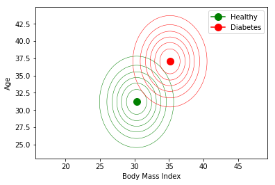
Now, if I am a patient with a body mass index of 40, and 33 years old, which decision will make this classifier? And if I am 25 years old? Think first, or try to predict the result.

def print_diagnosis(body_mass, age):
    distance_diabetes = mahalanobis_dist(mean_diabetes, [body_mass, age], sigma)
    distance_healthy = mahalanobis_dist(mean_healthy, [body_mass, age], sigma)
    if distance_diabetes > distance_healthy:
        print('Diagnostic for body mass', body_mass, 'and age', age, 'is: healthy')
    else:
        print('Diagnostic for body mass', body_mass, 'and age', age, 'is: diabetes')
        
print_diagnosis(40,33)
print_diagnosis(40,25)

3.2 - Using scikit-learn

The documentation for Naive Bayes in sklearn can be reached here and here for the Gaussian case.

The simplicity with which we can apply the Naive Bayes classifier to our data with sk-learn speaks by itself:

from sklearn.naive_bayes import GaussianNB
clf = GaussianNB()
clf.fit(features_reduced, labels)

print(clf.predict([40, 33]))
print(clf.predict([40, 25]))

Read (and fix)the warning!

from sklearn.naive_bayes import GaussianNB
data= np.array([40, 33]).reshape(1,-1)
print(clf.predict(data))

data= np.array([40, 25]).reshape(1,-1)
print(clf.predict(data))

Observe also how easily we can generalize to dealing with all the features with little effort:

clf_all = GaussianNB()
clf_all.fit(features, labels)

print(clf.predict(np.array([40, 33]).reshape(1,-1)))
print(clf.predict(np.array([40, 25]).reshape(1,-1)))

4.- Linear Regression: a (tiny) bit of theory

In order to give an example of a problem different than classification, we are going to use Linear Regression. The idea of Linear Regression is simply to find the linear function that best explains our labeled data. Hence, in the one-dimensional case, we will be finding simply a line; in case we have two features, this will be a plane, etc.

Regardless of the dimension, every linear space can be described as:

$$L(\mathbf{x},\theta) = \theta_0 + \theta_1 \cdot x_1 + \ldots +\theta_N x_N$$

and the set of parameters $\theta=(\theta_0, \theta_1, \ldots, \theta_N)$ are the numbers that specify the subspace. For instance, in the one-dimensional case, we would have:

$$L(\mathbf{x},\theta) = \theta_0 + \theta_1 \cdot x_1$$

which is the equation of a straight line.

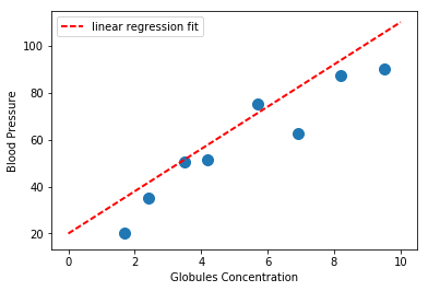
We could then have a dataset for linear regression that has the following appearance:

features = np.array([1.7, 2.4, 3.5, 4.2, 5.7, 6.9, 8.2, 9.5])
targets = np.array([20.2, 35.3, 50.4, 51.2, 75.2, 62.7, 87.3, 90.1])

import matplotlib.pyplot as plt
plt.scatter(features, targets, s=100);
plt.xlabel('Globules Concentration')
plt.ylabel('Blood Pressure')
plt.show()

Finding a linear model that solves this problem would imply specifying $\theta_0, \theta_1$ in the above equation. For instance we can specify $\theta_0 = 20$, $\theta_1 = 1$ and see if it fits our data properly:

theta_0 = 20
theta_1 = 9
x = np.linspace(0, 10, 100)
y = theta_0 + theta_1*x
plt.plot(x,y, 'r--', lw = 2, label = 'linear regression fit')
plt.scatter(features, targets, s=100);
plt.xlabel('Globules Concentration')
plt.ylabel('Blood Pressure')
plt.legend()

If you trust in your model, you can now use it to predict blood pressure out of, for instance, a patient with globules concentration of $x=5$:

new_patient_concentration = 5.0
predicted_blood_pressure = theta_0 + theta_1*new_patient_concentration
print(predicted_blood_pressure)

As mentioned above, we are going to discuss deeply this kind of models both for classification and regression in the theoretical lectures. However, it is useful for you to see how does sk-learn handle this kind of problems, which we do below.

5.- Linear Regression Using scikit-learn

As you may be expecting, you can easily accomplish this task with sk-learn:

from sklearn.linear_model import LinearRegression

# Create Model
model = LinearRegression()

After instantiating a linear regressor, we can fit it in the same way as we fit a classifier:

# Fit Model
model.fit(features.reshape(-1, 1), targets)

And we are now ready for making new predictions:

# Fit Model
model.predict(5)

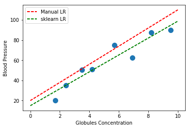
We can compare the fit computed by sk-learn with the one we manually computed above:

# Fit Model
predicted_by_sklearn = model.predict(x.reshape(-1,1))
plt.plot(x,y, 'r--', lw = 2, label = 'Manual LR')
plt.plot(x,predicted_by_sklearn, 'g--', lw = 2, label = 'sklearn LR')
plt.scatter(features, targets, s=100);
plt.xlabel('Globules Concentration')
plt.ylabel('Blood Pressure')
plt.legend()

6.- Homework

---

6. Homework

6.1 - Graded Homework: Training and Testing data.

First part

It is important to test your trained models on new data that has not been used for training. Otherwise you could be overly optimistic on its performance. For that, we typically save some training data and use them in the end only. In the same way as we refer to the data used to learn a model as training set, we refer to the independent data you hold apart from the begining as test set.

Sk-learn provides functionality for easily doing this operation. Look up in google or wherever for this sk-learn method, and apply it to split the full Pima Indian dataset from section 3.1 into a training set ($75\%$ of the data) and a test set. Train a Naive Bayes classifier on the training set, and then predict the appearence of diabetes on every element of the test set. Store your predictions in a numpy array with two columns, allocating in the first one the predictions.

Print your predictions on the test set together with the correct labels using the function provided below.

def print_predictions_and_labels(array_preds_labels):
    for predicted_pair in array_preds_labels:
        prediction = predicted_pair[0]
        label = predicted_pair[1]
        print('Prediction', prediction, 'Label', label)

preds_and_labels = np.array([[1,1],[0,1],[1,0]])
print_predictions_and_labels (preds_and_labels)       

Second part

The simplest way you can evaluate a binary classifier is by means of accuracy, which is defined as the number of data points (in your test set!) that were correctly classified over number of total data points.

Again, sklearn comes to help you. Look for a function (contained in sklearn.metrics) that can give you the accuracy score your classifier achieves. Read the documentation, undestand how is that function used, and use it to print the accuracy.

Note: There is an alternative to that function. Every fitted classifier in sklearn has a method of its own that you can use to output accuracy on a separate test set. This method is named score. Use it to find out your accuracy in the test set, and verify that it is the same as in the above case.

6.2 - Graded Homework: Simple Linear Regression

First part

We now consider a different dataset, but related also to diabetes. In this case we want to do linear regression. The dataset is described here, and contains ten variables (features): age, sex, body mass index, average blood pressure, and six blood serum measurements. These were extracted from a set of $442$ diabetes patients, and the target prediction is given by certain (unspecified) quantitative measure of disease progression one year after baseline.

This dataset comes already with sklearn, so you can load it from the sklearn.datasets module. We can load the dataset into a tuple containing two numpy arrays as follows:

diabetes_dataset = datasets.load_diabetes(return_X_y=True)

The following two lines will fit a linear regressor to this dataset:

model = LinearRegression()
model.fit(diabetes_dataset[0], diabetes_dataset[1])

Your goal now is to fit again the regressor, but this time split first the dataset into a training and a test set, and train the model only on the training data, reserving $30\%$ of your test set apart.

Second part

Evaluating regression models requires different error measures than accuracy, since we do not have now an idea of well/wrong classified. In this case, you can observe the mean square error in your test set, defined as you may have expected:

$$MSE = \sum_{i=1}^N(\mathrm{target}_i - \mathrm{prediction}_i)^2$$

But to begin with, you need to compute the predictions of your model on the test data:

diabetes_test_predictions = model2.predict(X_test)
type(diabetes_test_predictions)

Now you can use the MSE error provided for you by the sklearn.metrics module under the name mean_squared_error. Import it and use it to compute the error. Note that you will need to feed it the predictions and the actual values.

from sklearn.metrics import mean_squared_error

mean_squared_error(y_test, diabetes_test_predictions)

In this case, the precise error value does not help too much on itself, since we do not have a reference value to compare with. However, notice that it can be useful to compare with other regression models.

6.3 - Ungraded Homework: k-nearest neighbor classification

k-nearest neighbor is a very intuitive classifier that works as follows: Suppose you have a dataset with examples given by:

$${\mathbf{x}^i, y_i} \ \ \mathrm{for} \ \ 1\leq i \leq m,$$

described by $n$ features $\mathbf{x}^i = (x^i_0,x^i_1, \ldots, x^i_n)$, with labels $y_i$.

Given a new example $\mathbf{x}^{new} = (x^{new}_0,x^{new}_1, \ldots, x^{new}_n)$, your model will assign to it a label by comparing the distance between $\mathbf{x}^{new}$ and all your training examples, and the decision is made depending on the label of the closest $k$ neighbors.

In this case, we are going to fix $k=3$. So, if the lowest distances were given by, e.g., $\mathbf{x}^{12}$, $\mathbf{x}^{57}$, and $\mathbf{x}^{62}$, and you have that $y^{12} = 0, y^{57} = 1, y^{62} = 1$, then the new sample receives a prediction of $y^{new}=1$.

In order to implement k-nearest neighbors, you need a definition of “closest”, which means that you need a definition of distance between to $n$-dimensional points. We will be using the standard Euclidean distance, defined as the norm of the difference between the two points:

$$\mathrm{dist}(\mathrm{p}, \mathrm{q}) = |\mathrm{p} - \mathrm{q}|_2 = \sqrt{(p_1-q_1)^2 + (p_2-q_2)^2 + \ldots (p_n-q_n)^2 + }$$

This distance can be easily implemented, or you can use the norm function from numpy.linalg library:

def distance(x,y):
    return np.linalg.norm(x-y)

p = np.array([0,0])
q = np.array([2,0])

print('Distance between (0,0) and (2,0) is', distance(p,q))

p = np.array([0,0,0,0])
q = np.array([2,2,0,0])
print('Distance between (0,0) and (2,0) is', distance(p,q))

First part: Implementation from scratch

I am completely aware that this could be challenging if you are not too familiar with numpy. However, one of the best ways to learn both coding and the inner mechanisms of machine learning models is to try to implement them from scratch. No matter if your implementation is the most inefficient in the world, no matter if it is not even free of Python errors, I just want you to try implementing the idea described above. Submit whatever your attempt to solve this is, I don’t mind if you feel what you do is not the best implementation in the world or even if you think you are ashamed of it. Please submit!

We are going to use the same reduced version of the Iris dataset as in section 1.d. This is loaded for you again in the next code snippet. Try to implement code for classifying a new example given by $\mathbf{x}^{new} = (3.5,2.5,2.5,0.75)$.

If you succeed implementing this, then split the training and test set (30$\%$ for the test set) and compute the accuracy error from all the examples in the test set.

Second part: KNN with sk-learn

Now investigate how can you replicate the above, but this time with the sklearn library.

7. Sources and References

[1] Theoretical lessons for DACO, in your moodle.

[2] It could be useful to watch this short video on generative models.

[3] The second lecture of the Udacity’s online course Intro to Machine Learning, accessible here

[4] You can find a nice overview and implementation of k-NN in Kevin Zakka’s blog. Be aware that he is making more us of the pandas library than we do.